
The SUBTOTAL function is incredibly versatile, and the name is misleading since it can perform any of 11 different calculations not just finding totals. The particular calculation is controlled by using a specific value for one of the arguments, which we will describe below. There are two main reasons why the SUBTOTAL function is so popular:
- It performs calculations on filtered data.
- It calculates visible cells (you have the option of including all the cells).
Before we look at the example let us quickly review the SUBTOTAL function syntax.
The SUBTOTAL function’s syntax has two required arguments:
=SUBTOTAL(function argument, ref1, [ref2], […])
The first argument identifies the type of calculation we are interested in doing. This could be a sum, an average, a minimum, a maximum, a count, etc. Excel assigns a number to each of these types of calculation. The values 1 through 11 give us calculations that include all of the cells in a given data range including the hidden values, while values 101 through 111 give us calculations that include only the cells that are visible in a data range. Ref1, ref2, etc. refers to cells or ranges that we want to subtotal. Figure 1 presents the list of the function arguments:
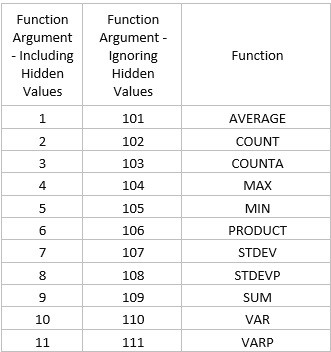
Figure 1
In this article, we will look at the example of the SUBTOTAL function used for the data set for the top 25 car sales by country in 2020 (https://www.factorywarrantylist.com/car-sales-by-country.html) (Figure 2).
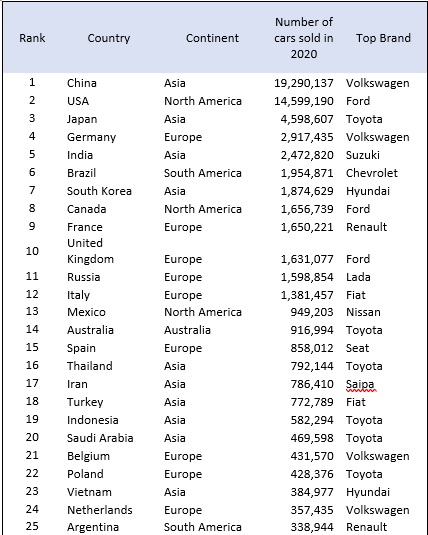
Figure 2
We would like to know:
- How many top brand vehicles were sold on each continent?
- How many vehicles were sold of each brand?
Let’s address the first question: How many top brand vehicles were sold on each continent?
The easiest way to answer the above question is to sort data by continent and then use the SUBTOTAL SUM function.
Step 1: Apply the Filter command in the top row of the data set (Figure 3).
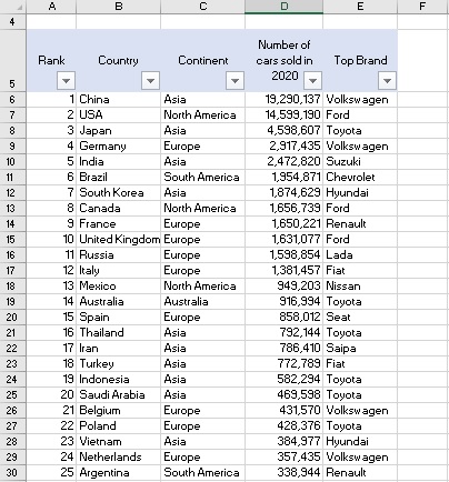
Figure 3
Step 2: Sort the data set by the continents (column C) (Figure 4).
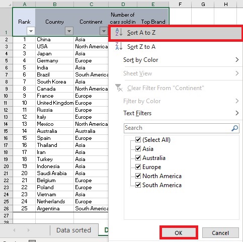
Figure 4
Figure 5 shows the data set sorted by continent.
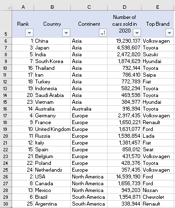
Figure 5
Step 3: Before we use the SUBTOTAL function, we need to do a bit of setup, specifically we need to insert blank rows at the locations that we what subtotals. If we want to know the number of cars sold for each continent, we need to separate each continent with an empty row. See Figure 6.
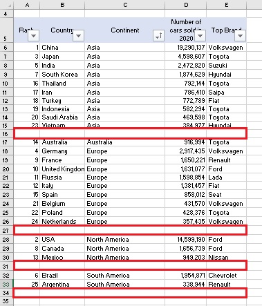
Figure 6
Step 4: Select cell D16 and type the SUBTOTAL SUM function for all cars sold in Asia:
=SUBTOTAL(109,D6:D15).
You can use 9 or 109 as the argument of the function since in this example we don’t have hidden values.
Repeat this step for the sum of cars sold in Europe, North and South America (Figure 7).
The function for Europe will look like: =SUBTOTAL(109,D18:D26). Notice that this function doesn’t include Australia which is in row 17.
The function for North America will look like: =SUBTOTAL(109,D28:D30)
The function for South America will look like: =SUBTOTAL(109,D32:D33)
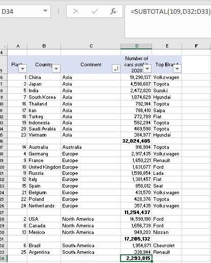
Figure 7
Excel has two functions which can sum the numbers in a range, the SUBTOTAL function discussed above, and the SUM function. A useful difference for generating a grand total is that when we have SUBTOTALs in the range of a different SUBTOTAL function, the results of the included SUBTOTAL functions are ignored with the effect that the data are totaled correctly. The SUM function will actually include the total of other SUM functions in a range, so a grand total is not as easy to calculate.
The larger the number of subtotals we calculate the more time we need to set up the calculations using the SUBTOTAL Function. There is a faster method – the SUBTOTAL Command located on the Data tab in the Outline group. It automatically creates groups and uses one of the 11 common functions like SUM, PRODUCT, AVERAGE, MIN, and MAX to summarize data as shown in Figure 1. The question “How many vehicles were sold of each brand?” will be addressed using the SUBTOTAL Command in the follow-up article https://windsongtraining.ca/an-example-of-using-the-subtotal-command-in-excel/

Leave A Comment