
For many of us, Microsoft Excel might be either the only tool, or a favourite tool, that we have available for data analysis. Excel can work with large amounts of data, but there are limitations on how much data we can load into a worksheet. In particular, the maximum number of rows in a single worksheet is just over one million; 1,048,576 to be precise.
In this post, we have a sample data file with 5 columns and 2,299,502 rows. Loading this into an Excel worksheet will load just under half of the file. The file has a header row so including that, the worksheet can hold the first 1,048,576 rows of the data file. The zipped data file can be downloaded here if you wish to experiment with this yourself. The compressed file is 11 MB in size and inflates to 77 MB when unzipped. We will attempt to load this data file into a Microsoft 365 Excel (64-bit, 2022 version) worksheet to see how Excel behaves when under the pressure of too much data.
Fig. 1 shows rows at the top of the .txt file, including the header line. Note that commas are used as delimiters so the filename could equivalently use a .csv extension (for “comma separated values”). There are 5 columns in the data file with either integer, date or text data types.
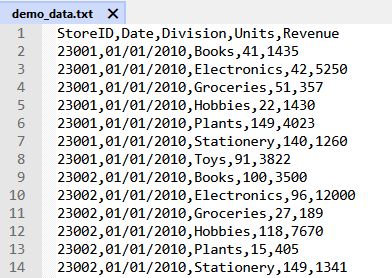
Fig. 1 – First few rows of a sample data file
Fig. 2 shows the file entries around row 1048576. This row is the maximum number that we can load into an Excel worksheet. The data file contains just over double that number of rows and we will see how Excel behaves when we try to load the whole file into a worksheet.
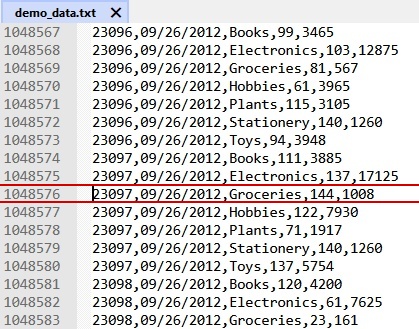
Fig. 2 – demo data file around line 1,048,576.
To load the data file we will use the Power Query data importer located on the Data tab. Open Excel and select the Data tab. In the Get & Transform Group, click on the From Text/CSV command as shown in Fig. 3 to open the file browser.

Fig. 3 – Power Query text import command.
Find the appropriate file on your computer and select “Import” to have Excel begin reading the file into Excel. We don’t want to use any of Power Query’s tools to make changes to the data as we import, so select the “Load” drop-down arrow and click on “Load To”. This brings up the “Import Data” dialog shown in Fig. 4.
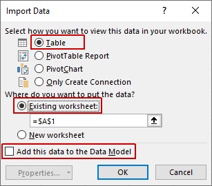
Fig. 4 – Power Query Data Import dialog.
Choose the radio button for “Table” in the top section. If you have an empty worksheet with cell A1 selected, you can choose “Existing worksheet” for where you want to put the data, otherwise select “New worksheet”. Ensure that “Add this data to the Data Model” is not checked, as shown in Fig. 4. Click on “OK” to start the data import. The Queries & Connections area will show a progressive count of rows loaded – this can take a while for large data files.

Fig. 5 – Progressive count of uploaded rows.
The current sample data file on my computer took about 20 seconds to load, your mileage will vary.
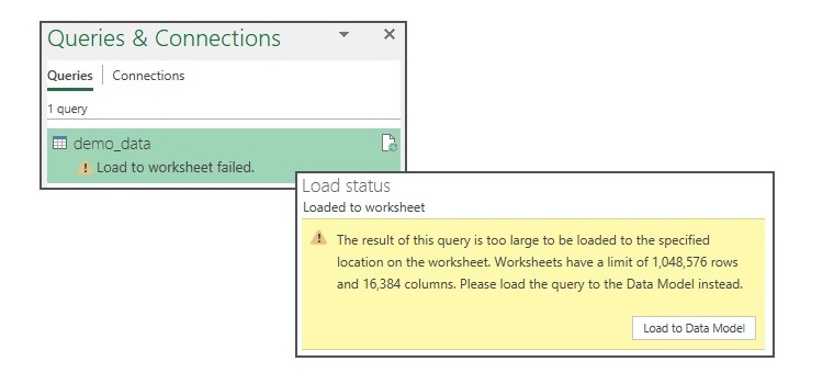
When the number of rows in the source data file is larger than the number of rows that a worksheet can hold, we get the “Load to worksheet failed.” message as shown in Fig. 6.
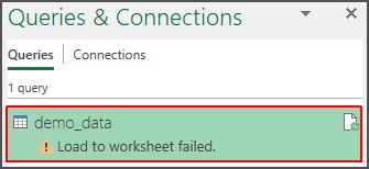
Fig. 6 – Load to worksheet failed message.
We can see the last line that was loaded into the worksheet in Fig. 7 which we can compare to the input text shown in Fig. 2.
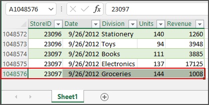
Fig. 7 – The last data file lines loaded to the worksheet.
The data importer simply truncates the data at 1048576 rows and discards the rest. If we are to perform analysis on the full data set, we could load sections into three different worksheets for this sample data set, but of course analysis becomes a bit awkward. Fortunately, we can load all the data into the Excel Data Model now and work with it directly. This will be the subject of next articles.


Leave A Comment