Excel has 4 functions that allow us to find a value in a column or row, and return a value from a corresponding column or row. The lookup functions can be very useful and are easy to understand when they provide an exact match for a search item. In addition to exact matches, the functions can provide “approximate” matching, and this can be a bit harder to understand. We are going to look at an example where the structure of the approximate match is natural, and if we keep this in mind, the lookup functions can be powerful tools.
The currently available lookup functions in Excel are:
- Lookup() – the oldest lookup function – from VisiCalc in 1979
- vLookup() – appeared in Lotus 1-2-3 in 1983
- hLookup() – appeared in Lotus 1-2-3 in 1983
- xLookup() – newest lookup function, currently available with Excel in Microsoft 365
Microsoft included versions of Lookup(), vLookup() and hLookup() in version 1 of Excel (released in 1985) for compatibility with other spreadsheet software products. The initial version of Excel was only available on the Macintosh computer, and it took until 1987 for Excel version 2 to be available on the PC.
There are other functions that can be used in combination to look up values, for example Index() and Match(), but we won’t be considering them in this article.
Depending on the particular lookup function you are using, you may specify the range of cells to work with as either a vector or an array. The post Ranges in Excel provides a brief explanation if you would like a refresher.
Table 1 provides a summary of some interesting features of Excel’s Lookup() functions – interesting for this post, anyway. Note that Lookup() and xLookup() can both use vector ranges and all the functions can use array ranges. The details vary for how they work, so the Excel help is very useful.
| Function | Vector Range | Array Range | Sorted | Approximate Match | Exact Match | Return Multiple |
|---|---|---|---|---|---|---|
| Lookup() | Yes | Yes | Yes | Default | No | |
| vLookup() | Yes | Yes, for approximate match | Default | Yes | No | |
| hLookup() | Yes | Yes, for approximate match | Default | Yes | No | |
| xLookup() | Yes | Yes | Yes, for approximate match | Yes | Default | Yes |
Table 1: Excel Lookup Function Properties
All the lookup functions can do what is referred to as an “approximate match”, which requires that the range you are searching through is sorted, otherwise you will get unpredictable results. The approximate match can be confusing when we first see it so we are going to look at the details of how it works.
The Excel Lookup() function has the following syntax:
Lookup(lookup_value, lookup_vector, [result_vector])
where the Lookup() function is going to try to find the “lookup_value” in the range “lookup_vector” and then return a corresponding value in the “result_vector”. For example, Fig. 1 demonstrates using the Lookup() function to find the scientific name for Meerkat.
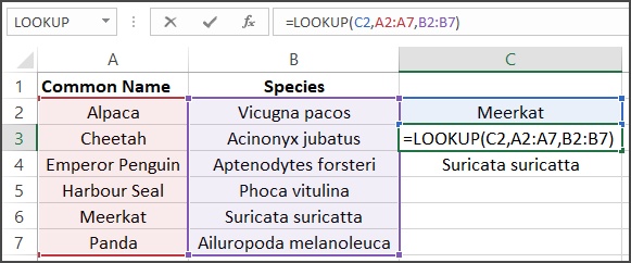
Fig. 1: The Excel Lookup() Function
The common names for some animals are listed in column A, and their corresponding scientific names are in column B. The list of animals in column A is sorted alphabetically for the Lookup() function to work correctly. The Lookup() function is shown in cell C3: the first parameter is what we are looking for, in this case “Meerkat”, which is found in cell C2. The vector range A2:A7 is where we are searching for “Meerkat”, and the range B2:B7 holds the values that the Lookup() function will return and display in cell C3. Cell C4 is a copy of C3 and shows the result of the Lookup() function which will be displayed in cell C3.
Excel’s help documentation for Lookup() states that:
- the values in the lookup_vector (the range that we are searching in) must be sorted in ascending order
- uppercase and lowercase text are equivalent – Lookup() is not case sensitive
- if Lookup() can’t find the lookup_value (what we are searching for), the function matches the largest value that is less than the lookup_value – we will clarify this below …
- if the lookup_value is smaller than the smallest value in the lookup_vector Lookup() will return #N/A
All of Excel’s Lookup functions are able to do an exact match, and except for Lookup() itself, we can specify that we only want an exact match. When we do an approximate match, it’s important to be clear about why it works as it does. For this, we are going to look at a simple table of tax rates in Fig. 2.
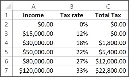
Fig. 2: Simple Tax Rates
In our simplified model of income tax rates shown in Fig. 2, if someone’s income is less than $15,000, they pay no income tax. If the income is between $15,000 and $30,000, there is 0% tax on the first $15,000, and 12% tax on the balance above $15,000. Someone who makes exactly $30,000 will pay no tax on the first $15,000 and 0.12x$15,000 = $1,800 for the next $15,000 for a total tax of $1,800 in tax for the year. Just to belabor the point a bit more, someone with an income of $50,000 will pay $1,800 in tax for the first $30,000 and then 0.18x$20,000=$3,600 for a total of $1,800+$3,600=$5,400 in income tax for the year. Fig. 3 shows a scatter plot of the Total Tax calculated against income for the tax model for Fig. 2.
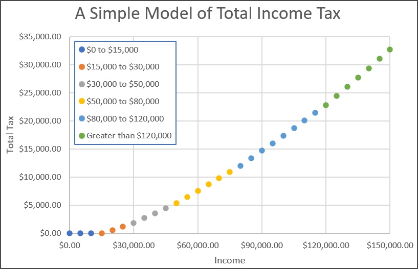
Fig. 3: Income Tax as a Function of Income for our Model
The calculations are easy enough when we have nice round numbers to calculate, but remember that in 1979, these calculations were generally done by hand. That year, VisiCalc was released and it had a Lookup() function that allowed us to find values in a tax table and have the computer do this calculation for us. This tax table lookup is what the Lookup function was made for.
In Fig. 4 we have some examples of using the Lookup() function to find the tax rate for a given income with our tax model from Fig. 2. Column F of Fig. 4 shows the values that we are going to look for in our tax table. Column G displays the value returned, and column H is a text version of the Lookup() function used in column G. Note that the commands in column H are surrounded by quotation marks to display the command – the actual output of the command (without quotation marks) is shown in column G.
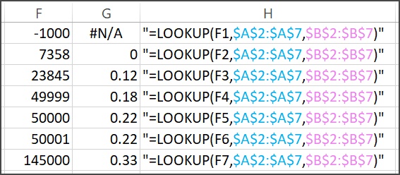
Fig. 4: Using the Lookup() function
If we look for a value smaller than the smallest value in the lookup range, Lookup() returns #N/A. We’ve searched for an income of -$1000 which is below the smallest value in the range A2:A7 and we get exactly what we are supposed to – no tax applies to a negative income and this probably indicates an error. Look closely at what happens with an income around $50,000. When the income is slightly less that $50,000, $49,999 in this example, Lookup() returns the tax rate value for $30,000. This is what approximate match does! For an income of $50,000, the match is exact, and a tax rate of 22% is returned. For $50,001 the match is approximate again and the tax rate returned is for $50,000. When we go to values larger than the largest in our tax table the approximate match returns the largest tax rate. In the context of the tax table, this behaviour of the Lookup() function makes sense.
Excel’s other lookup functions also do an approximate match the same way. In Fig. 5 we see vLookup() used to find the same values in the tax model from Fig. 2. The search range looks different because vLookup() and hLookup() require array ranges. In order to make this example look as similar as possible to the Lookup() example we are only using the two column range A2:B7 with the “$” signs inserted to make absolute references. The last parameter to vLookup(), the “2” tells vLookup to return the matched value from the second column of the range, that is from B2:B7.

Fig. 5: vLookup()
In Fig. 5, the values we search for are in column J, and the returned values are in column K. Column L shows the function used in column K. Note that hLookup() is the horizontal version of vLookup, so the range would involve 2 rows and 6 columns.
In Fig. 6, we see the same searches done with the xLookup() function. This example is using the vector ranges just as the Lookup() example did. An important difference with xLookup() is that matches are exact by default. The parameter “-1” tells xLookup() to do an approximate match and match the lower value, just as the Lookup() function does. It is possible to have xLookup() match the higher value in the search range, but that would be incorrect in the current example – see Excel’s documention for xLookup() for details.
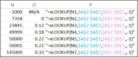
Fig. 6: xLookup()
In Fig. 6, the values we search for are in column N, and the returned values are in column O. Column P shows the function used in column O.
The examples of Excel’s lookup functions shown in Figures 4, 5 and 6 all behave the same way. In the context of a tax table lookup the behaviour of the approximate match is straighforward to understand and consistent across the functions.
Exact matches are easy to understand, either we find the value or we don’t. When we do an approximate lookup, we may get unexpected results if we don’t have a clear idea of what the function is doing. This is especially true if we are doing searches in a range that isn’t sorted, or is alphabetic. When working with Excel’s lookup functions, I suggest keeping this example in mind if you are in doubt about what the function is doing.
Leave A Comment