
In this article we will look at using Excel and the matrix multiply function MMULT, along with the TRANSPOSE function. We will go through an example using a formula and then go through the same example with a linear algebra perspective. This article assumes the reader has a basic knowledge of linear algebra, specifically dot product and matrix multiply. Using Linear Algebra techniques in Excel can be quite useful and efficient.
Consider the following example. Suppose we have a fictitious business that sells sweets and cakes. It is the end of April and we would like to know our Year To Date sales for each month. In the example spread sheet (see in Fig. 1) locations B3 to B8 contain the unit prices for each of the product types, and locations D3 to G8 contain the recorded amount of unit sales for each month:
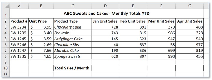
Fig. 1: Sample Data Set
Again look at Figure 1. In cell D10 we would like to know the total sales for January. This would be 728 Chocolate Cakes at $3.95 each, 743 Brownies at $3.40 each, and so on. Totals for the other months February to April we want in cells E10 to G10.
Method 1: Using a Formula
To find the total for January, starting with location D10, we could use the following formula (see Fig. 2):
=$B$3*D3 + $B$4*D4 + $B$5*D5 + $B$6*D6 + $B$7*D7 + $B$8*D8.
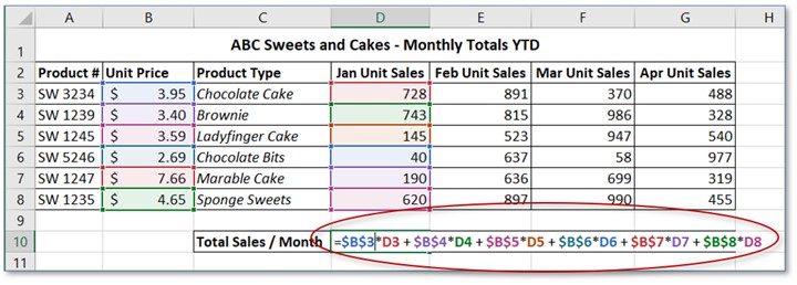
Fig. 2: Sample Data Set showing the formula used to calculate the total sales for January
This will give us a result, in D10, of $10,368.35 (see Fig. 3):
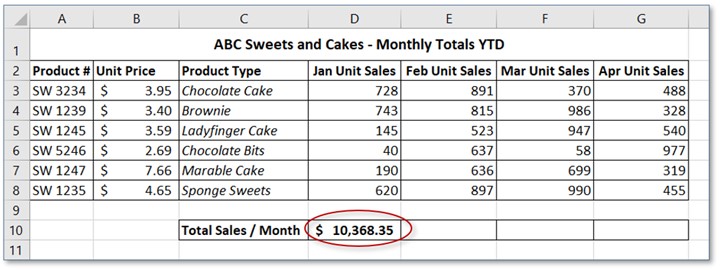
Fig. 3: Sample Data Set showing the total sales for January
Next, see Figure 4, we simply use the fill handle for cells E10, F10 and G10; and we’ll get the results. (Note that we used absolute referencing in the formula, see figure 2, for column B values so that they wouldn’t change when we use the fill handle.):
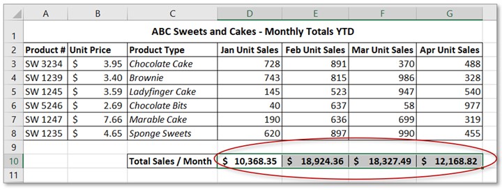
Fig. 4: Sample Data Set showing total sales for the four months
Method 2: Using the Matrix Multiply Function Along with the Transpose Function
Let’s look at the formula, see Figure 2, again:
=$B$3*D3 + $B$4*D4 + $B$5*D5 + $B$6*D6 + $B$7*D7 + $B$8*D8
It has the form of a dot product of two 6 dimensional vectors. The Unit Prices, B3 to B8 could be thought of as a vector; and the Unit Sales for each month, D3 to G8, could be thought of as a matrix. We just need to transform the Unit Prices to be a horizontal vector instead of vertical one, before we can do a matrix multiply. That is, in Excel, the first argument on the left needs to be a row vector.
We will need both the TRANSPOSE and MMULT functions to get the needed answers; and we’ll use the handy Insert Function command to help us out. To begin, let’s start over with the sample data. Select cell D10, as show in Figure 5, and click the “Insert Function” command. It is available on the Formulas Tab and also on the formula bar:
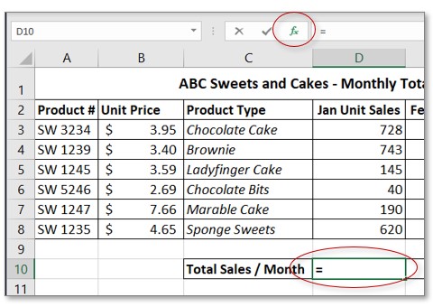
Fig. 5: Selecting the Insert Function command
In the Insert Function dialog box, as seen in Figure 6, type in “matrix multiply” in the “Search for a function” area and click on “Go”:
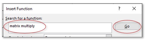
Fig. 6: Details of the top part of the Insert Function dialog box
The bottom part of the dialog box should show you the function name (see Figure 7). Click on MMULT if it is not already selected, then click on “OK”:
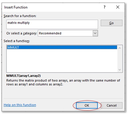
Fig. 7: Full details of using the Insert Function dialog box
The Function Arguments dialog box will show up next, see Figure 8:
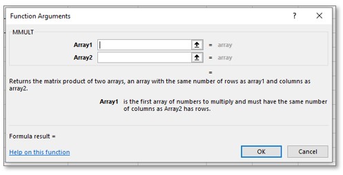
Fig. 8: Function Arguments dialog box for the MMULT function
For the first argument, labeled “Array1” in the dialog box, we want to use locations B3 to B8. However, we will need to transpose it first. We need B3 to B8 as a horizontal array instead of a vertical one. We can actually nest the TRANSPOSE function in the first argument of the MMULT function. In the “Array1” box type in: TRANSPOSE(B3:B8). Note that the dialog box gives a preview of the values it will use for the function on the right side of the input box. (See Figure 9):
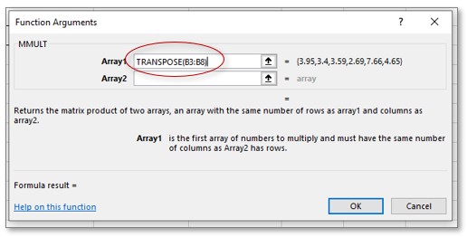
Fig. 9: Function Arguments dialog box for MMULT showing the first argument
For the second argument, “Array2”, we just need the location of the Unit Sales (See Fig. 10). So, either click and drag over location D3 to G8, or type in D3:G8, then click on OK:
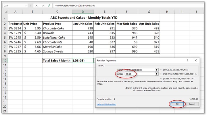
Fig. 10: Function Arguments dialog box for MMULT showing the second argument
The results follow, see Figure 11. Note that the values for locations E10, F10 and G10 were automatically filled in for us. (If you have a current Microsoft 365 subscription you can just click on the OK; otherwise press Ctrl+Shift+Enter):
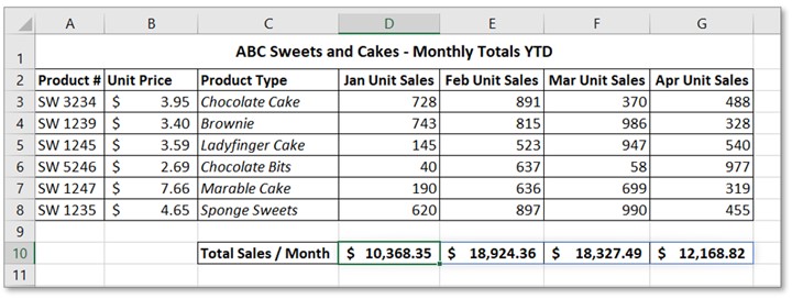
Fig. 11: Final Results
Both methods are acceptable. However, the use of basic linear algebra techniques, with Excel’s MMULT and TRANSPOSE functions, allows for an alternative method, well suited for substantial amounts of data. Using Linear Algebra techniques in Excel can be quite useful and efficient.

Leave A Comment