Recently we posted an article in which we looked at the example of the SUBTOTAL command (https://windsongtraining.ca/an-example-of-using-the-subtotal-command-in-excel/). We used this command to analyse the data set for the top 25 car sales by country in 2020 (https://www.factorywarrantylist.com/car-sales-by-country.html) (Figure 1).
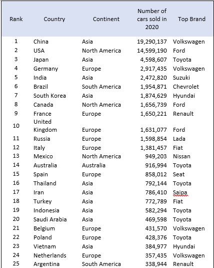
Figure 1
In this post we would like to use a Pivot Table for the same data set and address the same two questions that we had while using the SUBTOTAL command:
- How many top brand vehicles were sold on each continent?
- How many vehicles were sold of each brand?
It only takes a few seconds to answer each question when using Pivot Table. We assume here that the reader knows how to use PivotTables. An introductory article about the use of PivotTables is coming soon.
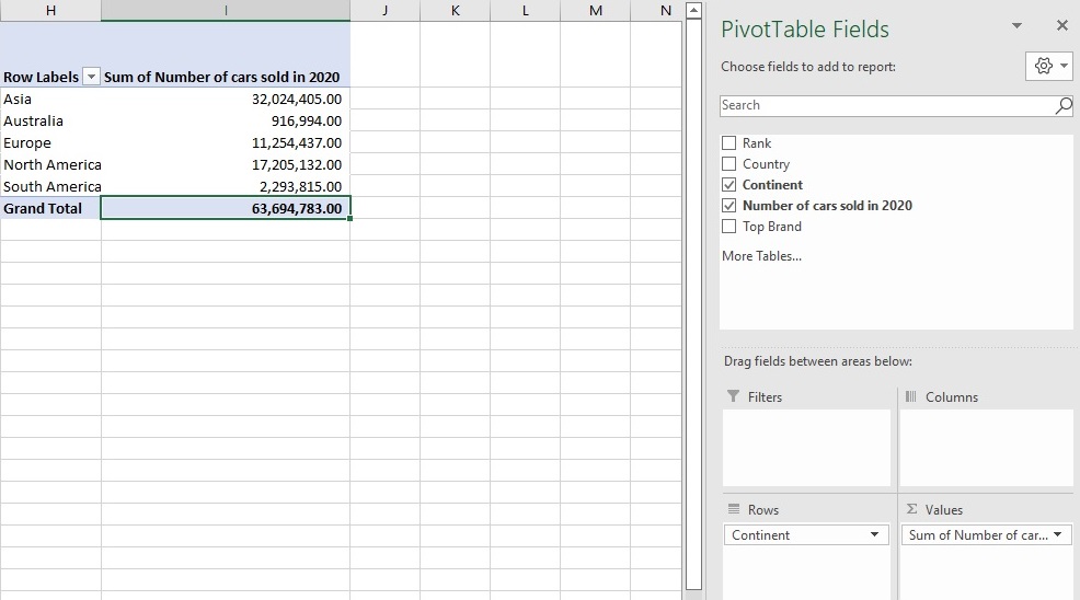
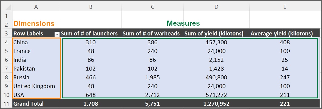
Figure 2: How many top brand vehicles were sold on each continent?
Let’s look now at the PivotTable used to answer the second question.
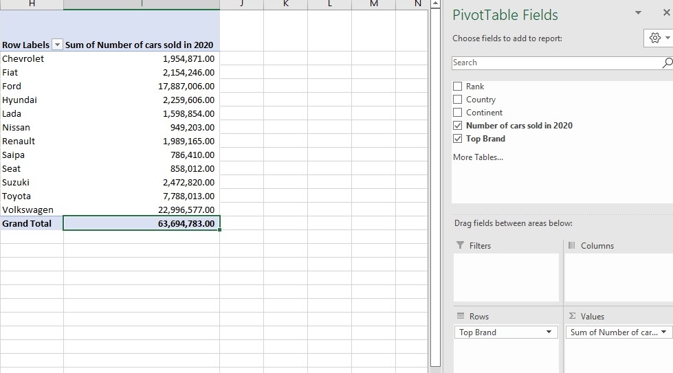
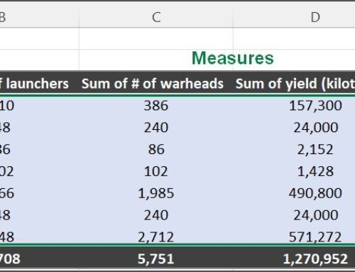
Figure 3: How many vehicles were sold of each brand?
There are two main advantages of using PivotTable over the SUBTOTAL command:
- We don’t have to sort data by a particular element (continent and top brand in our example) to get the SUBTOTAL for this element.
- All the subtotals are summarized in the PivotTable versus the subtotals appearing below each element in the table.
Leave A Comment